sSNAPPY: Singel Sample directioNAl Pathway Perturbation analYsis
Wenjun Nora Liu
Dame Roma Mitchell Cancer Research Laboratories, Adelaide Medical School, University of Adelaidewenjun.liu@adelaide.edu.au Source:
vignettes/sSNAPPY.Rmd
sSNAPPY.RmdIntroduction
This vignette demonstrates how to use the package
sSNAPPY to compute directional single sample pathway
perturbation scores by incorporating pathway topologies, utilize sample
permutation to test the significance of individual scores and compare
average pathway activities across treatments.
The package also provides a function to visualise overlap between pathway genes contained in perturbed biological pathways as network plots.
To get ready
Installation
The package sSNAPPY can be installed using the package
BiocManager
if (!"BiocManager" %in% rownames(installed.packages()))
  install.packages("BiocManager")
# Other packages required in this vignette
pkg <- c("tidyverse", "magrittr", "ggplot2", "cowplot", "DT")
BiocManager::install(pkg)
BiocManager::install("sSNAPPY")
install.packages("htmltools")
Load data
The example dataset used for this tutorial can be loaded with
data() as shown below. It’s a subset of data retrieved from
Singhal
H et al. 2016, where ER-positive primary breast cancer tumour
tissues collected from 12 patients were split into tissue fragments of
equal sizes for different treatments.
For this tutorial, we are only looking at the RNA-seq data from
samples that were treated with vehicle, R5020(progesterone) OR
E2(estrogen) + R5020 for 48 hrs. They were from 5 different patients,
giving rise to 15 samples in total. A more detailed description of the
dataset can be assessed through the help page
(?logCPM_example and ?metadata_example).
data(logCPM_example)
data(metadata_example)
# check if samples included in the logCPM matrix and metadata dataframe are identical
setequal(colnames(logCPM_example), metadata_example$sample)
## [1] TRUE
# View sample metadata
datatable(metadata_example,  filter = "top")
sSNAPPY workflow
Compute weighted single-sample logFCs (ssLogFCs)
It is expected that the logCPM matrix will be filtered to remove
undetectable genes and normalised to correct for library sizes or other
systematic artefacts, such as gene length or GC contents, prior to
applying the sSNAPPY workflow. Filtration and normalisation
have been performed on the example dataset.
Before single-sample logFCs (ssLogFCs) can be computed, row names of
the logCPM matrix need to be converted to entrez ID. This
is because all the pathway topology information retrieved will be in
entrez ID. The conversion can be achieved through
bioconductor packages AnnotationHub and
ensembldb.
head(logCPM_example)To compute the ssLogFCs, samples must be in matching pairs. In our
example data, treated samples were matched to the corresponding control
samples derived from the same patients. Therefore the
groupBy parameter of the weight_ss_fc()
functions will be set to be “patient”.
weight_ss_fc() requires both the logCPM matrix and
sample metadata as input. The column names of the logCPM matrix should
be sample names, matching a column in the metadata. Name of the column
with sample name will be provided as the sampleColumn
parameter. The function also requires the name of the metadata column
containing treatment information to be specified. The column with
treatment information must be a factor with the control treatment set to
be the reference level.
#compute weighted single sample logFCs
weightedFC <- weight_ss_fc(logCPM_example, metadata = metadata_example,
                           groupBy  = "patient", sampleColumn = "sample",
                           treatColumn = "treatment")
The weight_ss_fc() function firstly computes raw
ssLogFCs for each gene by subtracting logCPM values of the control
sample from the logCPM values of treated samples for each patient.
It has been demonstrated previously that in RNA-seq data, lowly
expressed genes turn to have a larger variance, which is also
demonstrated by the plots below. To reduce the impact of this artefact,
weight_ss_fc also weights each ssLogFCs by estimating the
relationship between the variance in ssLogFCs and mean logCPM, and
defining the gene-wise weight to be the inverse of the predicted
variance of that gene’s mean logCPM value.
perSample_FC <- lapply(levels(metadata_example$patient), function(x){
    temp <- logCPM_example[seq_len(1000),str_detect(colnames(logCPM_example), x)]
    ratio <- temp[, str_detect(colnames(temp), "Vehicle", negate = TRUE)] - temp[, str_detect(colnames(temp), "Vehicle")]
}) %>%
    do.call(cbind,.)
aveCPM <- logCPM_example[seq_len(1000),] %>%
    rowMeans() %>%
    enframe(name = "gene_id",
            value = "aveCPM")
p1 <- perSample_FC %>%
    as.data.frame() %>%
    rownames_to_column("gene_id") %>%
    pivot_longer(cols = -"gene_id",
                 names_to = "name",
                 values_to = "logFC") %>%
    left_join(aveCPM) %>%
    ggplot(aes(aveCPM, logFC)) +
    geom_point() +
    labs(y = "sslogFC",
         x = "Average logCPM") +
    theme(
        panel.background = element_blank()
    )
p2 <- data.frame(
    gene_id = rownames(perSample_FC),
    variance = perSample_FC %>%
        apply(1,var)) %>%
    left_join(aveCPM) %>%
    ggplot(aes(aveCPM, variance)) +
    geom_point() +
    geom_smooth(method = "loess") +
    labs(y = "Variance in ssLogFCs",
         x = "Average logCPM") +
    theme(
        panel.background = element_blank()
    )
plot_grid(p1, p2)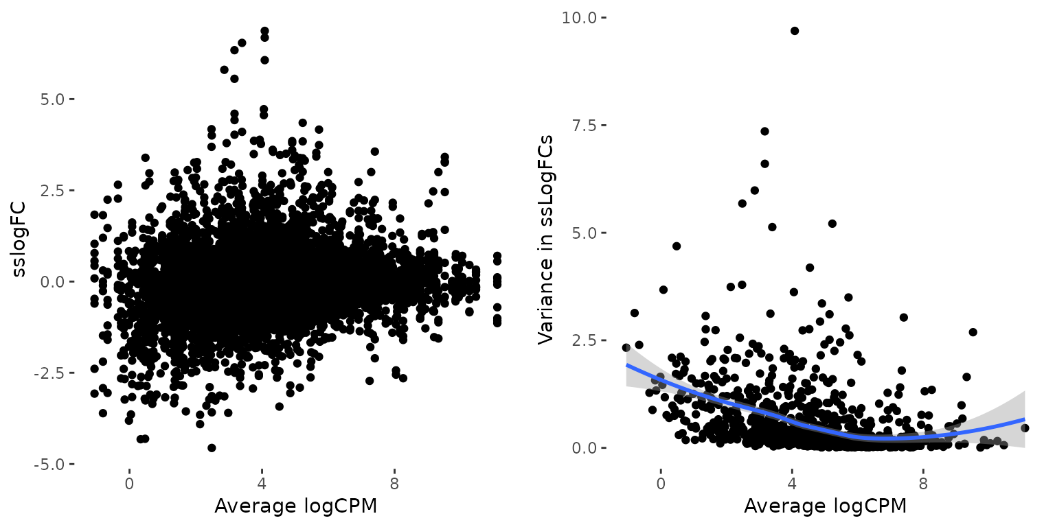
The output of the weight_ss_fc() function is a list with
two element, where one is the weighted ssLogFCs matrix and the other is
a vector of gene-wise weights.
Retrieve pathway topologies in the required format
sSNAPPY adopts the pathway perturbation scoring algorithm proposed in SPIA, which makes use of gene-set topologies and gene-gene interaction to propagate pathway genes’ logFCs down the topologies to compute pathway perturbation scores, where signs of scores reflect the potential directions of changes.
Therefore, pathway topology information needs to be firstly retrieved from your chosen database and converted to weight adjacency matrices, the format required to apply the scoring algorithm.
This step is achieved through a chain of functions that are part of
the grapghite,
which have been nested into one simple function in this package called
retrieve_topology(). The retrieve_topology
function now supports large lists of species and databases. Databases
that are currently supported for human are:
library(graphite)
graphite::pathwayDatabases() %>%
  dplyr::filter(species ==  "hsapiens") %>%
pander::pander()| species | database |
|---|---|
| hsapiens | kegg |
| hsapiens | panther |
| hsapiens | pathbank |
| hsapiens | pharmgkb |
| hsapiens | reactome |
| hsapiens | smpdb |
| hsapiens | wikipathways |
The retrieved topology information will be a list where each element corresponds a pathway. It’s recommended to save the list as a file so this step only needs to be performed once for each database.
This vignette chose KEGG pathways in humanh as an example.
gsTopology <- retrieve_topology(database = "kegg", species = "hsapiens")
head(names(gsTopology))
## [1] "kegg.Glycolysis / Gluconeogenesis"
## [2] "kegg.Citrate cycle (TCA cycle)"
## [3] "kegg.Pentose phosphate pathway"
## [4] "kegg.Pentose and glucuronate interconversions"
## [5] "kegg.Fructose and mannose metabolism"
## [6] "kegg.Galactose metabolism"If only selected biological processes are of interest to your research, it’s possible to only retrieve the topologies of those pathways by specifying keywords. For example, to retrieve all metabolism-related KEGG pathways:
gsTopology_sub <- retrieve_topology(
  database = "kegg",
  species = "hsapiens",
  keyword = "metabolism")
names(gsTopology_sub)
## [1] "kegg.Fructose and mannose metabolism"
## [2] "kegg.Galactose metabolism"
## [3] "kegg.Ascorbate and aldarate metabolism"
## [4] "kegg.Purine metabolism"
## [5] "kegg.Caffeine metabolism"
## [6] "kegg.Pyrimidine metabolism"
## [7] "kegg.Alanine, aspartate and glutamate metabolism"
## [8] "kegg.Glycine, serine and threonine metabolism"
## [9] "kegg.Cysteine and methionine metabolism"
## [10] "kegg.Arginine and proline metabolism"
## [11] "kegg.Histidine metabolism"
## [12] "kegg.Tyrosine metabolism"
## [13] "kegg.Phenylalanine metabolism"
## [14] "kegg.Tryptophan metabolism"
## [15] "kegg.beta-Alanine metabolism"
## [16] "kegg.Taurine and hypotaurine metabolism"
## [17] "kegg.Phosphonate and phosphinate metabolism"
## [18] "kegg.Selenocompound metabolism"
## [19] "kegg.Glutathione metabolism"
## [20] "kegg.Starch and sucrose metabolism"
## [21] "kegg.Amino sugar and nucleotide sugar metabolism"
## [22] "kegg.Glycerolipid metabolism"
## [23] "kegg.Inositol phosphate metabolism"
## [24] "kegg.Glycerophospholipid metabolism"
## [25] "kegg.Ether lipid metabolism"
## [26] "kegg.Arachidonic acid metabolism"
## [27] "kegg.Linoleic acid metabolism"
## [28] "kegg.alpha-Linolenic acid metabolism"
## [29] "kegg.Sphingolipid metabolism"
## [30] "kegg.Pyruvate metabolism"
## [31] "kegg.Glyoxylate and dicarboxylate metabolism"
## [32] "kegg.Propanoate metabolism"
## [33] "kegg.Butanoate metabolism"
## [34] "kegg.Thiamine metabolism"
## [35] "kegg.Riboflavin metabolism"
## [36] "kegg.Vitamin B6 metabolism"
## [37] "kegg.Nicotinate and nicotinamide metabolism"
## [38] "kegg.Lipoic acid metabolism"
## [39] "kegg.Retinol metabolism"
## [40] "kegg.Porphyrin metabolism"
## [41] "kegg.Nitrogen metabolism"
## [42] "kegg.Sulfur metabolism"
## [43] "kegg.Metabolism of xenobiotics by cytochrome P450"
## [44] "kegg.Drug metabolism - cytochrome P450"
## [45] "kegg.Drug metabolism - other enzymes"
## [46] "kegg.Carbon metabolism"
## [47] "kegg.2-Oxocarboxylic acid metabolism"
## [48] "kegg.Fatty acid metabolism"
## [49] "kegg.Nucleotide metabolism"
## [50] "kegg.Cholesterol metabolism"
## [51] "kegg.Central carbon metabolism in cancer"
## [52] "kegg.Choline metabolism in cancer"It is also possible to provide multiple databases’ names and/or multiple keywords.
gsTopology_mult <- retrieve_topology(
  database = c("kegg", "reactome"),
  species = "hsapiens",
  keyword = c("metabolism", "estrogen"))
names(gsTopology_mult)
## [1] "kegg.Fructose and mannose metabolism"
## [2] "kegg.Galactose metabolism"
## [3] "kegg.Ascorbate and aldarate metabolism"
## [4] "kegg.Purine metabolism"
## [5] "kegg.Caffeine metabolism"
## [6] "kegg.Pyrimidine metabolism"
## [7] "kegg.Alanine, aspartate and glutamate metabolism"
## [8] "kegg.Glycine, serine and threonine metabolism"
## [9] "kegg.Cysteine and methionine metabolism"
## [10] "kegg.Arginine and proline metabolism"
## [11] "kegg.Histidine metabolism"
## [12] "kegg.Tyrosine metabolism"
## [13] "kegg.Phenylalanine metabolism"
## [14] "kegg.Tryptophan metabolism"
## [15] "kegg.beta-Alanine metabolism"
## [16] "kegg.Taurine and hypotaurine metabolism"
## [17] "kegg.Phosphonate and phosphinate metabolism"
## [18] "kegg.Selenocompound metabolism"
## [19] "kegg.Glutathione metabolism"
## [20] "kegg.Starch and sucrose metabolism"
## [21] "kegg.Amino sugar and nucleotide sugar metabolism"
## [22] "kegg.Glycerolipid metabolism"
## [23] "kegg.Inositol phosphate metabolism"
## [24] "kegg.Glycerophospholipid metabolism"
## [25] "kegg.Ether lipid metabolism"
## [26] "kegg.Arachidonic acid metabolism"
## [27] "kegg.Linoleic acid metabolism"
## [28] "kegg.alpha-Linolenic acid metabolism"
## [29] "kegg.Sphingolipid metabolism"
## [30] "kegg.Pyruvate metabolism"
## [31] "kegg.Glyoxylate and dicarboxylate metabolism"
## [32] "kegg.Propanoate metabolism"
## [33] "kegg.Butanoate metabolism"
## [34] "kegg.Thiamine metabolism"
## [35] "kegg.Riboflavin metabolism"
## [36] "kegg.Vitamin B6 metabolism"
## [37] "kegg.Nicotinate and nicotinamide metabolism"
## [38] "kegg.Lipoic acid metabolism"
## [39] "kegg.Retinol metabolism"
## [40] "kegg.Porphyrin metabolism"
## [41] "kegg.Nitrogen metabolism"
## [42] "kegg.Sulfur metabolism"
## [43] "kegg.Metabolism of xenobiotics by cytochrome P450"
## [44] "kegg.Drug metabolism - cytochrome P450"
## [45] "kegg.Drug metabolism - other enzymes"
## [46] "kegg.Carbon metabolism"
## [47] "kegg.2-Oxocarboxylic acid metabolism"
## [48] "kegg.Fatty acid metabolism"
## [49] "kegg.Nucleotide metabolism"
## [50] "kegg.Estrogen signaling pathway"
## [51] "kegg.Cholesterol metabolism"
## [52] "kegg.Central carbon metabolism in cancer"
## [53] "kegg.Choline metabolism in cancer"
## [54] "reactome.Metabolism"
## [55] "reactome.Inositol phosphate metabolism"
## [56] "reactome.PI Metabolism"
## [57] "reactome.Phospholipid metabolism"
## [58] "reactome.Nucleotide metabolism"
## [59] "reactome.Sulfur amino acid metabolism"
## [60] "reactome.Glycosaminoglycan metabolism"
## [61] "reactome.Integration of energy metabolism"
## [62] "reactome.Keratan sulfate/keratin metabolism"
## [63] "reactome.Heparan sulfate/heparin (HS-GAG) metabolism"
## [64] "reactome.Glycosphingolipid metabolism"
## [65] "reactome.Lipoprotein metabolism"
## [66] "reactome.Chondroitin sulfate/dermatan sulfate metabolism"
## [67] "reactome.Porphyrin metabolism"
## [68] "reactome.Estrogen biosynthesis"
## [69] "reactome.Bile acid and bile salt metabolism"
## [70] "reactome.Non-coding RNA Metabolism"
## [71] "reactome.Metabolism of steroid hormones"
## [72] "reactome.Cobalamin (Cbl, vitamin B12) transport and metabolism"
## [73] "reactome.Metabolism of folate and pterines"
## [74] "reactome.Biotin transport and metabolism"
## [75] "reactome.Vitamin D (calciferol) metabolism"
## [76] "reactome.Nicotinate metabolism"
## [77] "reactome.Vitamin C (ascorbate) metabolism"
## [78] "reactome.Vitamin B2 (riboflavin) metabolism"
## [79] "reactome.Metabolism of water-soluble vitamins and cofactors"
## [80] "reactome.Metabolism of vitamins and cofactors"
## [81] "reactome.Vitamin B5 (pantothenate) metabolism"
## [82] "reactome.Carnitine metabolism"
## [83] "reactome.Metabolism of nitric oxide: NOS3 activation and regulation"
## [84] "reactome.Metabolism of Angiotensinogen to Angiotensins"
## [85] "reactome.alpha-linolenic (omega3) and linoleic (omega6) acid metabolism"
## [86] "reactome.Linoleic acid (LA) metabolism"
## [87] "reactome.alpha-linolenic acid (ALA) metabolism"
## [88] "reactome.Metabolism of amine-derived hormones"
## [89] "reactome.Arachidonic acid metabolism"
## [90] "reactome.Hyaluronan metabolism"
## [91] "reactome.Metabolism of ingested SeMet, Sec, MeSec into H2Se"
## [92] "reactome.Selenoamino acid metabolism"
## [93] "reactome.Peptide hormone metabolism"
## [94] "reactome.Defects in vitamin and cofactor metabolism"
## [95] "reactome.Defects in biotin (Btn) metabolism"
## [96] "reactome.Metabolism of polyamines"
## [97] "reactome.Diseases associated with glycosaminoglycan metabolism"
## [98] "reactome.Glyoxylate metabolism and glycine degradation"
## [99] "reactome.Peroxisomal lipid metabolism"
## [100] "reactome.Metabolism of proteins"
## [101] "reactome.Regulation of lipid metabolism by PPARalpha"
## [102] "reactome.Sialic acid metabolism"
## [103] "reactome.Sphingolipid metabolism"
## [104] "reactome.Metabolism of lipids"
## [105] "reactome.Fructose metabolism"
## [106] "reactome.Diseases of carbohydrate metabolism"
## [107] "reactome.Diseases of metabolism"
## [108] "reactome.Surfactant metabolism"
## [109] "reactome.Metabolism of fat-soluble vitamins"
## [110] "reactome.Pyruvate metabolism"
## [111] "reactome.Glucose metabolism"
## [112] "reactome.Creatine metabolism"
## [113] "reactome.Amino acid and derivative metabolism"
## [114] "reactome.Carbohydrate metabolism"
## [115] "reactome.Pyruvate metabolism and Citric Acid (TCA) cycle"
## [116] "reactome.Ketone body metabolism"
## [117] "reactome.RUNX1 regulates estrogen receptor mediated transcription"
## [118] "reactome.Metabolism of RNA"
## [119] "reactome.Metabolism of steroids"
## [120] "reactome.Phenylalanine and tyrosine metabolism"
## [121] "reactome.Aspartate and asparagine metabolism"
## [122] "reactome.Phenylalanine metabolism"
## [123] "reactome.Glutamate and glutamine metabolism"
## [124] "reactome.Fatty acid metabolism"
## [125] "reactome.Metabolism of cofactors"
## [126] "reactome.Triglyceride metabolism"
## [127] "reactome.Glycogen metabolism"
## [128] "reactome.Extra-nuclear estrogen signaling"
## [129] "reactome.Estrogen-dependent gene expression"
## [130] "reactome.Regulation of glycolysis by fructose 2,6-bisphosphate metabolism"
## [131] "reactome.Estrogen-stimulated signaling through PRKCZ"
## [132] "reactome.Estrogen-dependent nuclear events downstream of ESR-membrane signaling"
## [133] "reactome.Retinoid metabolism and transport"Score single sample pathway perturbation
Once the expression matrix, sample metadata and pathway topologies are all ready, gene-wise single-sample perturbation scores can be computed:
genePertScore <- raw_gene_pert(weightedFC$logFC, gsTopology)and summed to derive pathway perturbation scores for each pathway in each treated samples.
pathwayPertScore <- pathway_pert(genePertScore)
head(pathwayPertScore)
## sample score gs_name
## 1 E2+R5020_N2_48 0.006717358 kegg.EGFR tyrosine kinase inhibitor resistance
## 2 R5020_N2_48 0.006718738 kegg.EGFR tyrosine kinase inhibitor resistance
## 3 E2+R5020_N3_48 0.002785146 kegg.EGFR tyrosine kinase inhibitor resistance
## 4 R5020_N3_48 -0.004030015 kegg.EGFR tyrosine kinase inhibitor resistance
## 5 E2+R5020_P4_48 0.004087122 kegg.EGFR tyrosine kinase inhibitor resistance
## 6 R5020_P4_48 0.015609886 kegg.EGFR tyrosine kinase inhibitor resistanceGenerate null distributions of perturbation scores
To derive the empirical p-values for each single-sample perturbation scores and normalize the raw scores for comparing overall treatment effects, null distributions of scores for each pathway are generated through a sample-label permutation approach.
For each round of permutation, sample labels are randomly shuffled to derive the permuted ssLogFCs, which are then used to score pathway perturbation. We recommend performing a minimum of 1000 rounds of permutation, which means at least 8 samples are required.
The generate_permuted_scores() function does not require
sample metadata but the number of treatments in the study design,
including the control treatment, need to be specified. In this example
data, the number of treatmentS was 3 (Vehicle, E2, and E2+R5020).
The output of the generate_permuted_scores() function is
a list where each element is a vector of permuted perturbation scores
for a pathway.
The permutation step relies on the parallel computing feature
provided by BiocParallel.
You can choose to customize the parallel back-end or stick with the
default one returned by BiocParallel::bpparam(). Depending
on the size of the data, this step can take some time to complete. If
the sample size is large, we recommend users consider performing this
step on an HPC.
set.seed(123)
permutedScore <- generate_permuted_scores(
  expreMatrix  = logCPM_example,
  numOfTreat = 3, NB = 1000,
  gsTopology = gsTopology,
  weight = weightedFC$weight
)
Test significant perturbation on
single-sample level
After the empirical null distributions are generated, the median and
mad of each distribution will be calculated for each pathway to convert
the test single-sample perturbation scores derived from the
compute_perturbation_score() function to robust z-scores:
\[(Score - Median)/MAD\]
Two-sided p-values associated with each robust z-scores are also
computed and will be corrected for multiple-testing using a user-defined
approach. The default is fdr.
The normalise_by_permu() function requires the test
perturbation scores and permuted perturbation scores as input. Users can
choose to sort the output by p-values, gene-set names or sample
names.
normalisedScores <- normalise_by_permu(permutedScore, pathwayPertScore, sortBy = "pvalue")Since the permutation step takes a long time to run and the output is
too large to be included as part of the package, the results of the
normalise_by_permu step has been pre-computed and can be
loaded with:
load(system.file("extdata", "normalisedScores.rda", package = "sSNAPPY"))Pathways that were significant perturbed within individual samples are:
normalisedScores %>%
    dplyr::filter(adjPvalue < 0.05) %>%
    left_join(metadata_example) %>%
    mutate_at(vars(c("sample", "gs_name")), as.factor) %>%
    mutate_if(is.numeric, sprintf, fmt = '%#.4f') %>%
    mutate(Direction = ifelse(robustZ < 0, "Inhibited", "Activation")) %>%
    dplyr::select(
        sample, patient, Treatment = treatment,
        `Perturbation Score` = robustZ, Direction,
        `Gene-set name` = gs_name,
        `P-value` = pvalue,
        FDR = adjPvalue
    ) %>%
    datatable(
        filter = "top",
        options = list(
            columnDefs = list(list(targets = "Direction", visible = FALSE))
        ),
        caption = htmltools::tags$caption(
                  htmltools::em(
                      "Pathways that were significant perturbed within individual samples.")
              )
    ) %>%
    formatStyle(
        'Perturbation Score', 'Direction',
        color = styleEqual(c("Inhibited", "Activation"), c("blue", "red"))
    )
Visualise overlap between gene-sets as networks
To visualise significantly perturbed biological pathways as a
network, where edges between gene-sets reflect how much overlap those
two gene-sets share, we can use the plot_gs_network
function. The function can take normalise_by_permu()’s
output, or a subset of it as its direct input.
Nodes in the network plots could be colored by the predicted direction of perturbation (i.e.. sign of robust z-score):
pl <- normalisedScores %>%
    dplyr::filter(adjPvalue < 0.05) %>%
    droplevels() %>%
    split(f = .$sample) %>%
    lapply(function(x){
        mutate(x,
               status = ifelse(
                   robustZ > 0, "Activated", "Inhibited"))
    }) %>%
    lapply(
        plot_gs_network,
        gsTopology = gsTopology,
        colorBy = "status",
        gsLegTitle = "Direction of pathway Perturbation"
    ) %>%
    lapply(function(x){
        x + theme(
            panel.grid = element_blank(),
            panel.background = element_blank()
        ) })
plot_grid(
    plotlist = pl,
    labels = names(pl),
    label_size = 8,
    nrow = 1)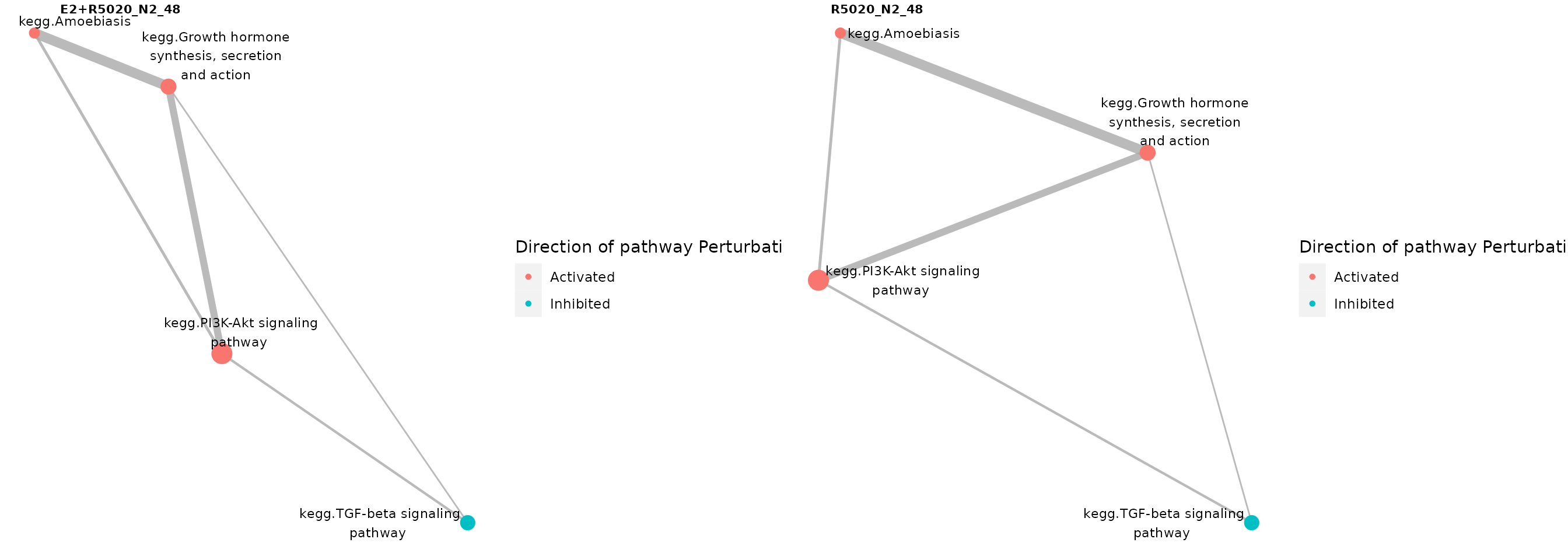
Pathways significantly perturbed in individual samples, where gene-sets were colored by pathways’ directions of changes.
Or p-values:
pl <- normalisedScores %>%
    dplyr::filter(adjPvalue < 0.05) %>%
    droplevels() %>%
    split(f = .$sample) %>%
    lapply(
        plot_gs_network,
        gsTopology = gsTopology,
        colorBy = "pvalue",
        color_lg_title = "P-value"
    ) %>%
    lapply(function(x){
        x + theme(
        panel.grid = element_blank(),
        panel.background = element_blank()
        ) })
plot_grid(
    plotlist = pl,
    labels = names(pl),
    label_size = 8,
    nrow = 1)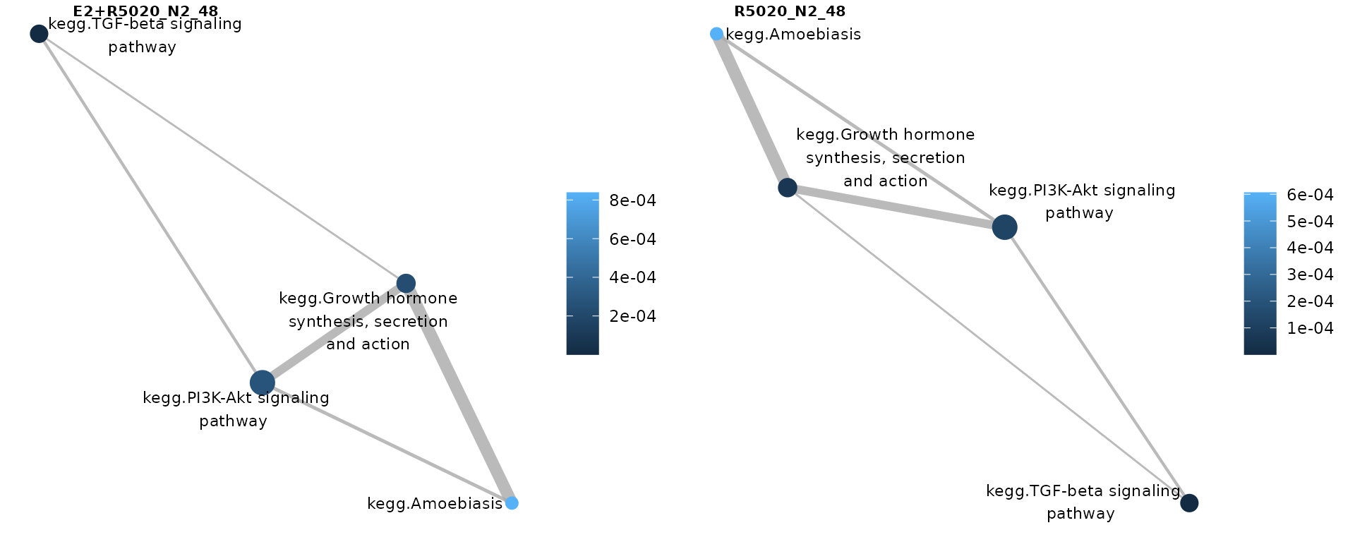
Pathways significantly perturbed in individual samples, where gene-sets were colored by pathways’ p-values
The function allows you to customize the layout, colour, edge
transparency and other aesthetics of the graph. More information can be
found on the help page (?plot_gs_network). The output of
the graph is a ggplot object and the theme of it can be
changed just as any other ggplot figures.
treatment-level
In addition to testing pathway perturbations at single-sample level, normalised perturbation scores can also be used to model mean treatment effects within a group, such as within each treatment group. An advantage of this method is that it has a high level of flexibility that allows us to incorporate confounding factors as co-factors or co-variates to offset their effects.
For example, in the example data-set, samples were collected from patients with different progesterone receptor (PR) statuses. Knowing that PR status would affect how tumour tissues responded to estrogen and/or progesterone treatments, we can include it as a cofactor to offset its confounding effect.
fit <- normalisedScores %>%
    left_join(metadata_example) %>%
    split(f = .$gs_name) %>%
    #.["Estrogen signaling pathway"] %>%
    lapply(function(x)lm(robustZ ~ 0 + treatment + PR, data = x)) %>%
    lapply(summary)
treat_sig <- lapply(
  names(fit),
  function(x){
    fit[[x]]$coefficients %>%
      as.data.frame() %>%
      .[seq_len(2),] %>%
      dplyr::select(Estimate, pvalue = `Pr(>|t|)` ) %>%
      rownames_to_column("Treatment") %>%
      mutate(
        gs_name = x,
        FDR = p.adjust(pvalue, "fdr"),
        Treatment = str_remove_all(Treatment, "treatment")
      )
  }) %>%
  bind_rows()
Results from the linear modelling revealed pathways that were on average perturbed due to each treatment:
treat_sig %>%
    dplyr::filter(FDR < 0.05) %>%
    mutate_at(vars(c("Treatment", "gs_name")), as.factor) %>%
    mutate_if(is.numeric, sprintf, fmt = '%#.4f') %>%
    mutate(Direction = ifelse(Estimate < 0, "Inhibited", "Activation")) %>%
    dplyr::select(
        Treatment, `Perturbation Score` = Estimate, Direction,
        `Gene-set name` = gs_name,
        `P-value` = pvalue,
        FDR
    ) %>%
    datatable(
        filter = "top",
        options = list(
            columnDefs = list(list(targets = "Direction", visible = FALSE))
        ),
        caption = htmltools::tags$caption(
                  htmltools::em(
                      "Pathways that were significant perturbed within each treatment group.")
              )
    ) %>%
    formatStyle(
        'Perturbation Score', 'Direction',
        color = styleEqual(c("Inhibited", "Activation"), c("blue", "red"))
    )
It is not surprising to see that the estrogen signalling pathway was significantly activated under both R5020 and E2+R5020 treatments.
Visualise genes’ contributions to pathway perturbation
If there’s a specific pathway that we would like to dig deeper into
and explore which pathway genes played a key role in its perturbation,
for example, activation of the “Ovarian steroidogenesis”, we can plot
the gene-level perturbation scores of genes that are constantly highly
perturbed or highly variable in that pathway as a heatmap using the
plot_gene_contribution() function.
From the heatmap below that we can see that the activation of this pathway was strongly driven by two genes: ENTREZID:3630 and ENTREZID:3479.
plot_gene_contribution(
    genePertMatr  = genePertScore$`kegg.Ovarian steroidogenesis`,
    # only plot genes with top 15 absolute mean gene-wise scores
    filterBy = "mean", topGene = 15
)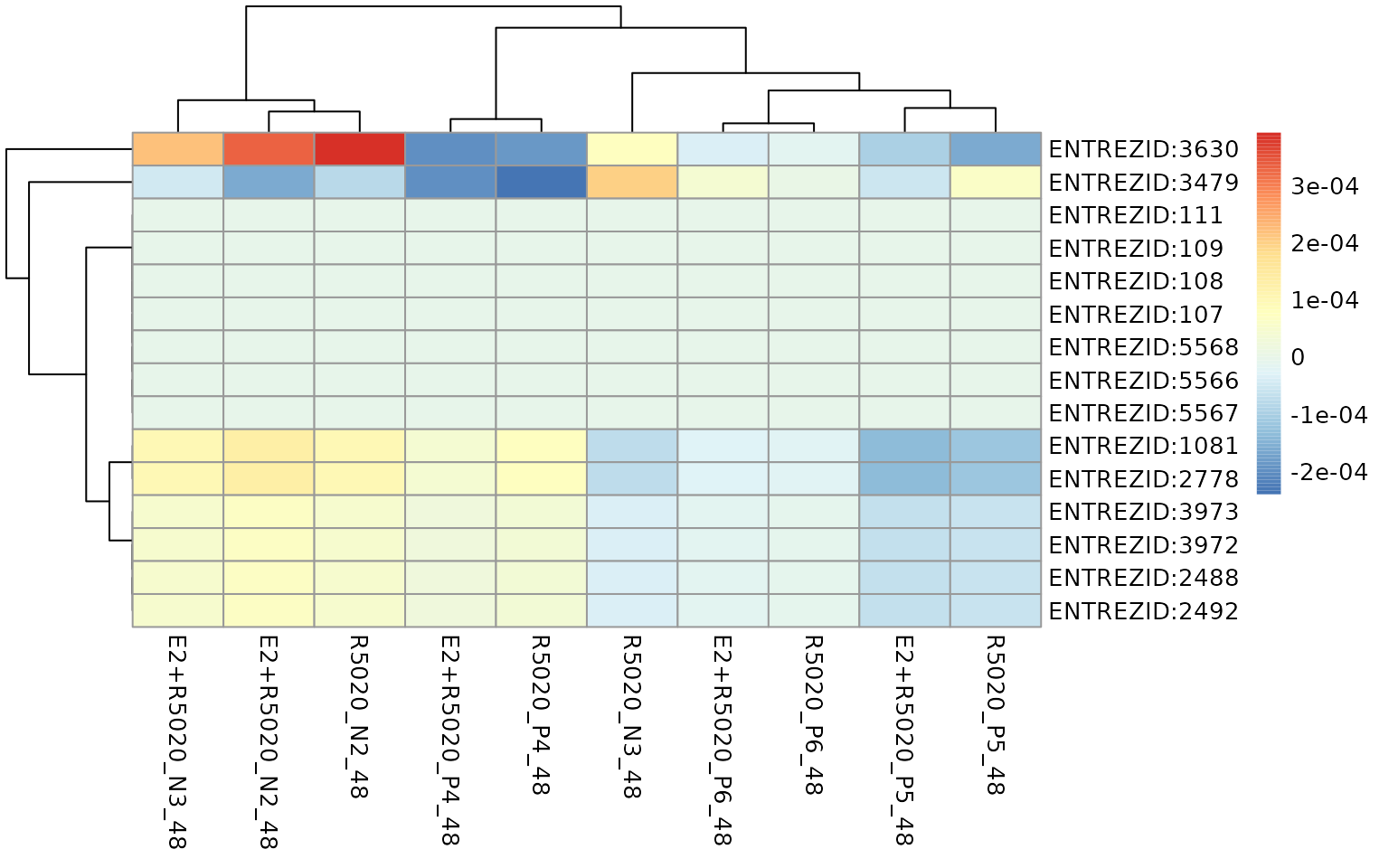
Gene-level perturbation scores of genes with top 15 absolute mean gene-wise perturbation scores in the Ovarian steroidogenesis gene-set.
By default, genes’ entrez IDs are used and plotted as row names,
which may not be very informative. So the row names could be overwritten
by providing a data.frame mapping entrez IDs to other
identifiers through the mapRownameTo parameter.
Mapping between different gene identifiers could be achieved through
the mapIDs() function from the Bioconductor package AnnotationDbi.
But to reduce the compiling time of this vignette, mappings between
entrez IDs and gene names have been provided as a
data.frame called entrez2name.
Note that if the mapping information was provided and the mapping was successful for some genes but not the others, only genes that have been mapped successfully will be plotted.
We can also annotate each column (ie. each sample) by the direction
of pathway perturbation in that sample or any other sample metadata,
such as their treaatments. To annotate the columns, we need to create an
annotation data.frame with desired attributes.
annotation_df <- pathwayPertScore %>%
    dplyr::filter(gs_name == "kegg.Ovarian steroidogenesis") %>%
    mutate(
        `pathway-level` =  ifelse(
            score > 0, "Activated", "Inhibited")
    ) %>%
    dplyr::select(sample, `pathway-level`) %>%
    left_join(
        .,  metadata_example %>%
            dplyr::select(sample, treatment),
        unmatched = "drop"
    )
Colors of the annotation could be customised through
pheatmap::pheatmap()’s annotation_colors
parameter.
load(system.file("extdata", "entrez2name.rda", package = "sSNAPPY"))
plot_gene_contribution(
    genePertMatr  = genePertScore$`kegg.Ovarian steroidogenesis`,
    annotation_df = annotation_df,
    filterBy = "mean", topGene = 15,
    mapEntrezID = entrez2name,
    annotation_colors = list(
        treatment = c(R5020 = "black", `E2+R5020` = "white"),
        `pathway-level` = c(Activated = "darkred", Inhibited = "lightskyblue"))
)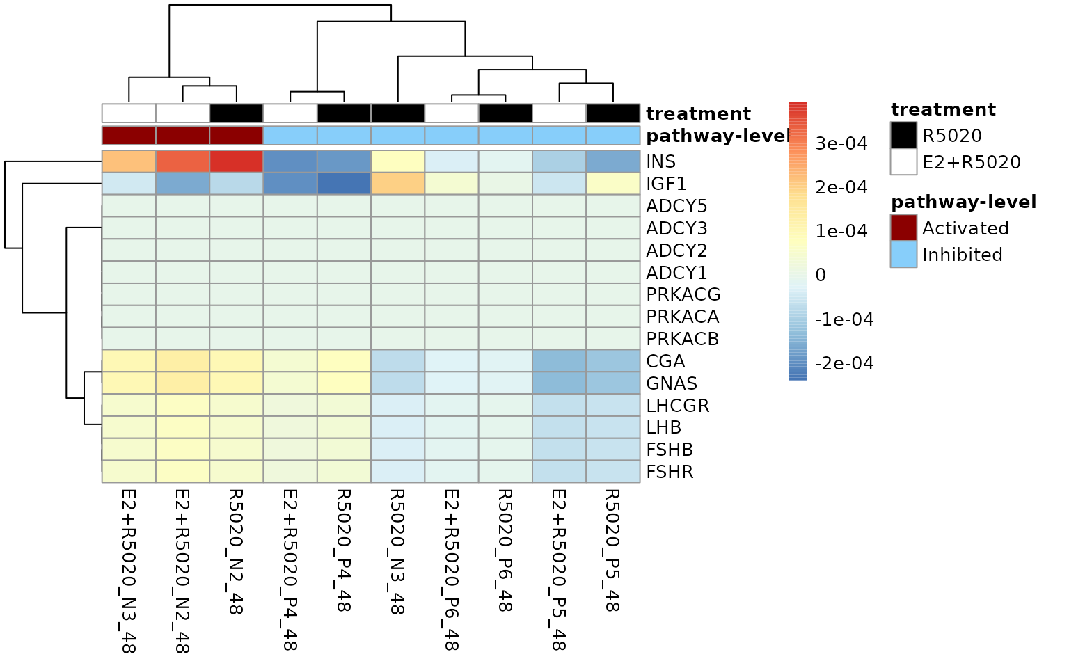
Gene-level perturbation scores of genes with top 15 absolute mean gene-wise perturbation scores in the Ovarian steroidogenesis gene-set.Genes playing the most important roles in pathway activation was INS, CGA, GNAS.
Visualise overlap between gene-sets as networks
Results of group-level perturbation can also be visualised using the
plot_gs_network() function.
treat_sig %>%
    dplyr::filter(FDR < 0.05, Treatment == "E2+R5020") %>%
    mutate(status = ifelse(Estimate > 0, "Activated", "Inhibited")) %>%
    plot_gs_network(
        gsTopology = gsTopology,
        colorBy = "status"
    ) +
    theme(
        panel.grid = element_blank(),
        panel.background = element_blank()
) 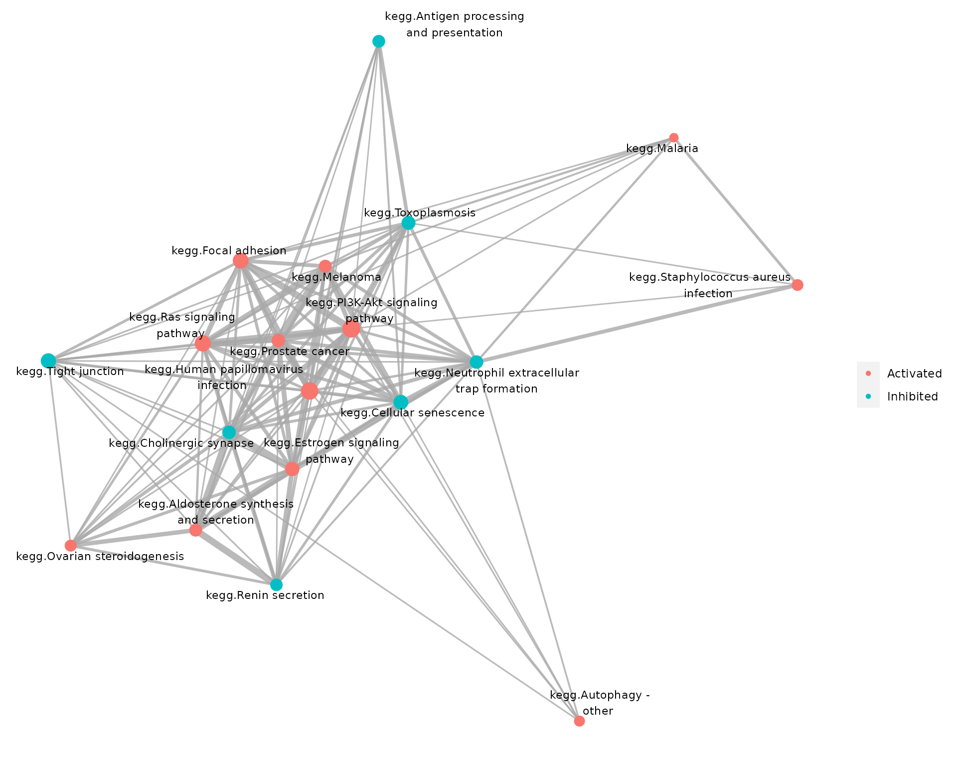
Pathways significantly perturbed by the E2+R5020 combintation treatment, where colors of nodes reflect pathways’ directions of changes.
By default, plot_gs_network() function does not include
nodes that are not connected to any other nodes, which could be turnt
off by setting the plotIsolated parameter to TURE.
Visualise community structure in the gene-set network
When a large number of pathways were perturbed, it is hard to answer
the question “What key biological processes were perturbed?” solely by
looking at all the pathway names. To solve that, we can use the
plot_community() function to apply a community detection
algorithm to the network we had above, and annotate each community by
the biological process that most pathways assigned to that community
belong to.
treat_sig %>%
    dplyr::filter(FDR < 0.05, Treatment == "E2+R5020") %>%
    plot_community(
        gsTopology = gsTopology,
        colorBy = "community",
        color_lg_title = "Community"
    ) +
    theme(panel.background = element_blank())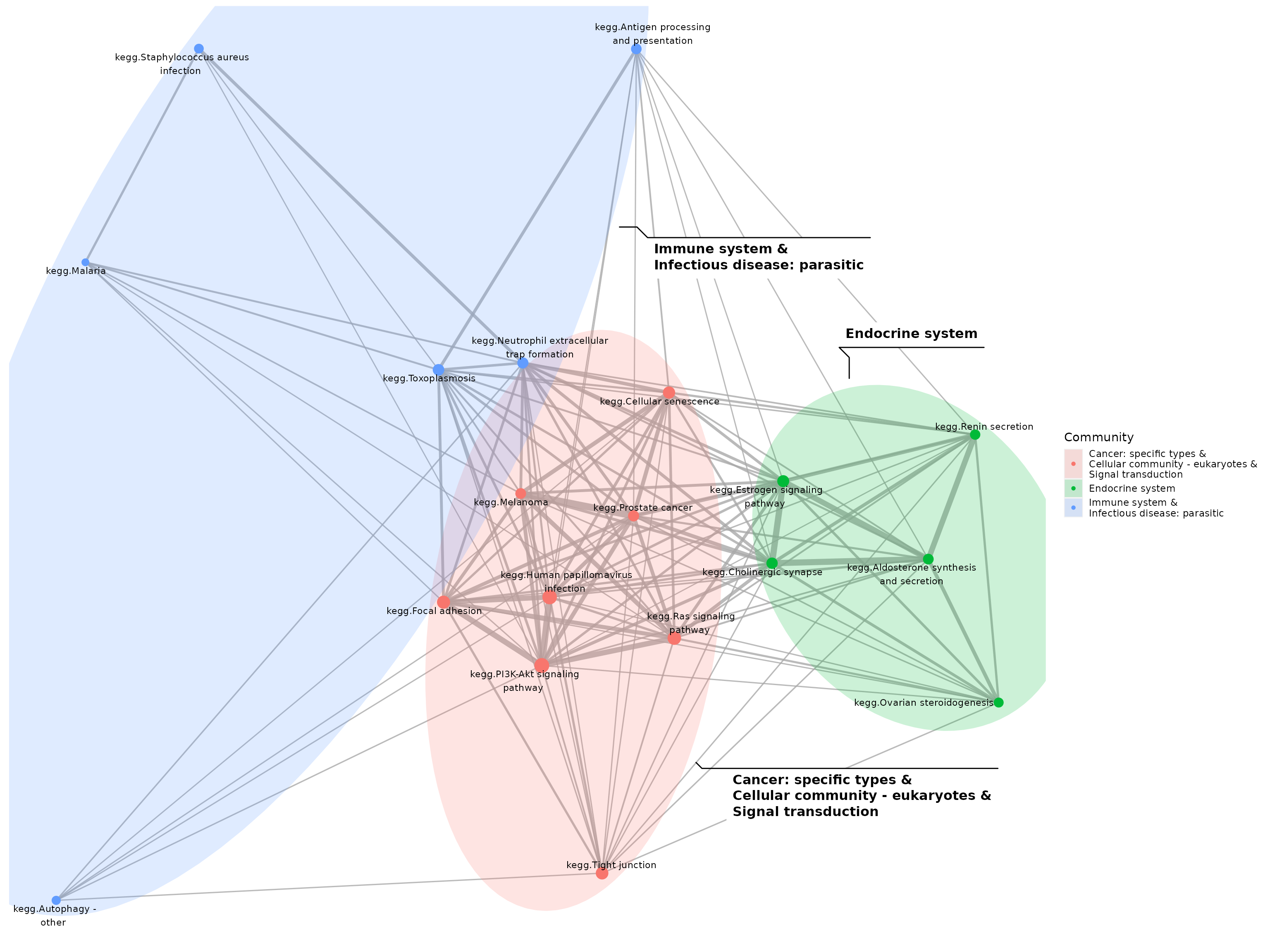
Pathways significantly perturbed by the E2+R5020 combintation treatment, annotated by the main biological processes each pathways belong to.
sSNAPPY was built in with categorisations of
KEGG pathways. But to annotate pathways retrieved from other
databases, customised annotation data.frame could be
provided through the gsAnnotation parameter.
Visualise genes included in perturbed pathways networks
If we want to not only know if two pathways are connected but also
the genes connecting those pathways, we can use the
plot_gs2gene() function instead:
treat_sig %>%
    dplyr::filter(FDR < 0.05, Treatment == "E2+R5020") %>%
    plot_gs2gene(
        gsTopology = gsTopology,
        colorGsBy = "Estimate",
        labelGene = FALSE,
        geneNodeSize  = 1,
        edgeAlpha = 0.1,
        gsNameSize = 2,
        filterGeneBy = 3
    ) +
    scale_fill_gradient2() +
theme(panel.background = element_blank()) 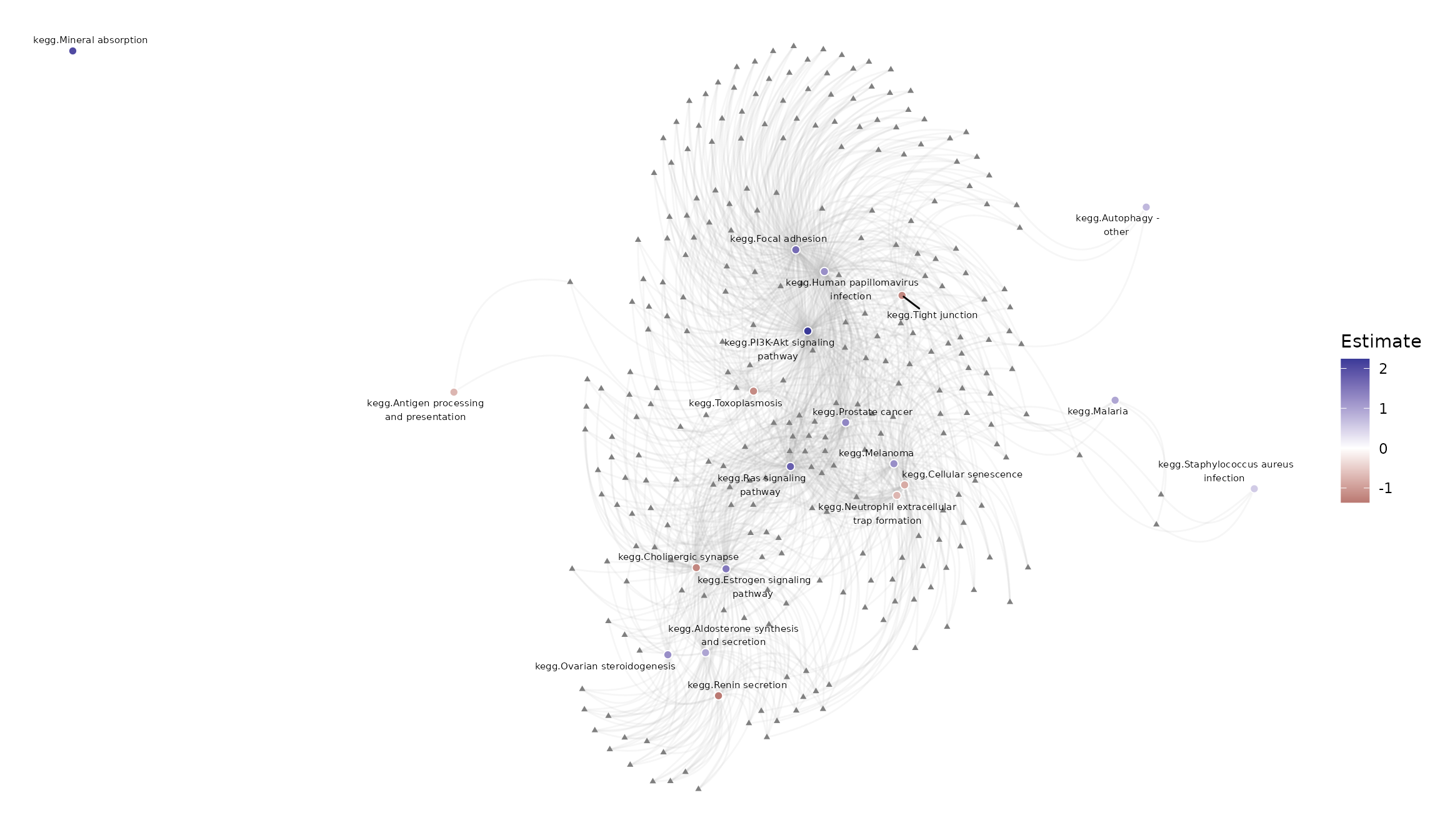
Pathways significantly perturbed by the E2+R5020 combintation treatment and genes contained in at least 3 of those pathways.
However, since there are a large number of genes in each pathway, the plot above was quite messy and it was unrealistic to plot all genes’ names. So it is recommend to filter pathway genes by their perturbation scores or logFCs.
For example, we can rank genes by the absolute values of their mean single-sample logFCs and only focus on genes that were ranked in the top 200 of the list.
meanFC <- weightedFC$logFC %>%
    .[, str_detect(colnames(.), "E2", negate = TRUE)] %>%
    apply(1, mean )
top200_gene <- meanFC %>%
    abs() %>%
    sort(decreasing = TRUE, ) %>%
    .[1:200] %>%
    names()
top200_FC <- meanFC %>%
    .[names(.) %in% top200_gene]
top200_FC  <- ifelse(top200_FC > 0, "Up-Regulated", "Down-Regulated")
When we provide genes’ logFCs as a named vector through the
geneFC parameter, only pathway genes with logFCs provided
will be plotted and gene nodes will be colored by genes’ directions of
changes. The names of the logFC vector must be genes’ entrez IDs in the
format of “ENTREZID:XXXX”, as pathway topology matrices retrieved
through retrieve_topology() always use entrez IDs as
identifiers.
However, it is not going to be informative to label genes with their
entrez IDs. So the same as the plot_gene_contribution()
function, we can provide a data.frame to match genes’
entrez IDs to our chosen identifiers through the
mapEntrezID parameter in the plot_gs2gene()
function too.
treat_sig %>%
    dplyr::filter(FDR < 0.05, Treatment == "E2+R5020") %>%
    mutate(status = ifelse(Estimate > 0, "Activated", "Inhibited")) %>%
    plot_gs2gene(
        gsTopology = gsTopology,
        colorGsBy = "status",
        geneFC = top200_FC,
        mapEntrezID = entrez2name,
        gsNameSize = 3
    ) +
    scale_fill_manual(values = c("darkred", "lightskyblue")) +
    scale_colour_manual(values = c("red", "blue")) +
    theme(panel.background = element_blank())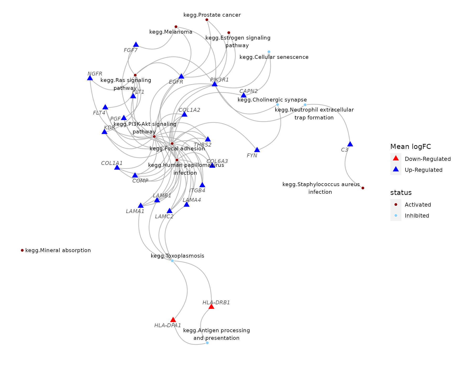
Pathways significantly perturbed by the E2+R5020 combintation treatment, and pathway genes with top 200 magnitudes of changes among all E2+R5020-treated samples. Both pathways and genes were colored by their directions of changes.
We can also filters genes’ by their contributions to a pathway
perturbations.To help with that, sSNAPPY provides an option
to rank genes’ perturbation scores within each sample for each
pathway.
If in a given pathway, both positive and negative gene-wise perturbation scores exist, positive and negative scores are ranked separately, where the larger a positive rank, the more the gene contributed to the pathway’s activation, and the smaller a negative rank, the more the gene contributed to the pathways’ inhibition.
geneRank <- rank_gene_pert(genePertScore, gsTopology)Depending on the biological question, it could be interesting to plot only the pathway genes with the same directions of changes as the pathway they belonged to, and ignoring those genes that were antagonizing the pathway perturbation.
References
- Sales G, Calura E, Cavalieri D, Romualdi C (2012). “graphite - a Bioconductor package to convert pathway topology to gene network.” BMC Bioinformatics. https://bmcbioinformatics.biomedcentral.com/articles/10.1186/1471-2105-13-20.
- Tarca, Adi Laurentiu et al. (2009). “A novel signaling pathway impact analysis.” Bioinformatics vol. 25,1 : 75-82. doi:10.1093/bioinformatics/btn577
Session Info
## R version 4.3.2 (2023-10-31)
## Platform: x86_64-pc-linux-gnu (64-bit)
## Running under: Ubuntu 22.04.3 LTS
##
## Matrix products: default
## BLAS:   /usr/lib/x86_64-linux-gnu/openblas-pthread/libblas.so.3
## LAPACK: /usr/lib/x86_64-linux-gnu/openblas-pthread/libopenblasp-r0.3.20.so;  LAPACK version 3.10.0
##
## locale:
##  [1] LC_CTYPE=C.UTF-8       LC_NUMERIC=C           LC_TIME=C.UTF-8
##  [4] LC_COLLATE=C.UTF-8     LC_MONETARY=C.UTF-8    LC_MESSAGES=C.UTF-8
##  [7] LC_PAPER=C.UTF-8       LC_NAME=C              LC_ADDRESS=C
## [10] LC_TELEPHONE=C         LC_MEASUREMENT=C.UTF-8 LC_IDENTIFICATION=C
##
## time zone: UTC
## tzcode source: system (glibc)
##
## attached base packages:
## [1] stats     graphics  grDevices utils     datasets  methods   base
##
## other attached packages:
##  [1] graphite_1.46.0   htmltools_0.5.6.1 DT_0.30           cowplot_1.1.1
##  [5] magrittr_2.0.3    lubridate_1.9.3   forcats_1.0.0     stringr_1.5.0
##  [9] dplyr_1.1.3       purrr_1.0.2       readr_2.1.4       tidyr_1.3.0
## [13] tibble_3.2.1      tidyverse_2.0.0   sSNAPPY_1.3.5     ggplot2_3.4.4
## [17] BiocStyle_2.28.1
##
## loaded via a namespace (and not attached):
##   [1] RColorBrewer_1.1-3          jsonlite_1.8.7
##   [3] farver_2.1.1                rmarkdown_2.25
##   [5] fs_1.6.3                    zlibbioc_1.46.0
##   [7] ragg_1.2.6                  vctrs_0.6.4
##   [9] memoise_2.0.1               RCurl_1.98-1.12
##  [11] S4Arrays_1.0.6              curl_5.1.0
##  [13] sass_0.4.7                  bslib_0.5.1
##  [15] htmlwidgets_1.6.2           desc_1.4.2
##  [17] plyr_1.8.9                  cachem_1.0.8
##  [19] igraph_1.5.1                lifecycle_1.0.3
##  [21] pkgconfig_2.0.3             Matrix_1.6-1.1
##  [23] R6_2.5.1                    fastmap_1.1.1
##  [25] GenomeInfoDbData_1.2.10     MatrixGenerics_1.12.3
##  [27] digest_0.6.33               colorspace_2.1-0
##  [29] AnnotationDbi_1.62.2        S4Vectors_0.38.2
##  [31] rprojroot_2.0.3             textshaping_0.3.7
##  [33] crosstalk_1.2.0             GenomicRanges_1.52.1
##  [35] RSQLite_2.3.2               org.Hs.eg.db_3.17.0
##  [37] labeling_0.4.3              fansi_1.0.5
##  [39] timechange_0.2.0            httr_1.4.7
##  [41] polyclip_1.10-6             abind_1.4-5
##  [43] mgcv_1.9-0                  compiler_4.3.2
##  [45] bit64_4.0.5                 withr_2.5.1
##  [47] pander_0.6.5                BiocParallel_1.34.2
##  [49] viridis_0.6.4               DBI_1.1.3
##  [51] ggforce_0.4.1               MASS_7.3-60
##  [53] rappdirs_0.3.3              DelayedArray_0.26.7
##  [55] tools_4.3.2                 glue_1.6.2
##  [57] nlme_3.1-163                grid_4.3.2
##  [59] reshape2_1.4.4              generics_0.1.3
##  [61] gtable_0.3.4                tzdb_0.4.0
##  [63] hms_1.1.3                   tidygraph_1.2.3
##  [65] utf8_1.2.4                  XVector_0.40.0
##  [67] BiocGenerics_0.46.0         ggrepel_0.9.4
##  [69] pillar_1.9.0                limma_3.56.2
##  [71] splines_4.3.2               tweenr_2.0.2
##  [73] lattice_0.21-9              bit_4.0.5
##  [75] tidyselect_1.2.0            locfit_1.5-9.8
##  [77] Biostrings_2.68.1           knitr_1.44
##  [79] gridExtra_2.3               bookdown_0.36
##  [81] IRanges_2.34.1              edgeR_3.42.4
##  [83] SummarizedExperiment_1.30.2 stats4_4.3.2
##  [85] xfun_0.40                   graphlayouts_1.0.1
##  [87] Biobase_2.60.0              matrixStats_1.0.0
##  [89] pheatmap_1.0.12             stringi_1.7.12
##  [91] yaml_2.3.7                  evaluate_0.22
##  [93] codetools_0.2-19            ggraph_2.1.0
##  [95] BiocManager_1.30.22         graph_1.78.0
##  [97] cli_3.6.1                   systemfonts_1.0.5
##  [99] munsell_0.5.0               jquerylib_0.1.4
## [101] Rcpp_1.0.11                 GenomeInfoDb_1.36.4
## [103] png_0.1-8                   parallel_4.3.2
## [105] ellipsis_0.3.2              pkgdown_2.0.7
## [107] blob_1.2.4                  bitops_1.0-7
## [109] viridisLite_0.4.2           scales_1.2.1
## [111] crayon_1.5.2                rlang_1.1.1
## [113] KEGGREST_1.40.1